Pulse programming and dynamical decoupling

Native gates are a set of carefully calibrated gates directly supported by the hardware. Behind the scenes, native gates themselves are implemented by analog control signals, or “pulses”, applied to the state of the qubits. Composing a program directly with pulse operations is called “pulse programming”, giving you even more control than native gates. For example, you can implement quantum operations directly with pulses in order to implement error suppression schemes such as dynamical decoupling, or error mitigation methods such as zero noise extrapolation. You can also improve the elementary operations by experimenting with novel custom gate implementations.

In this notebook, we demonstrate the pulse programming features of AutoQASM with two examples, one with a qubit idling program and one with dynamical decoupling which suppresses the error from qubit idling. These examples are taken from this blog post which composes programs using Amazon Braket SDK. This notebook shows you the examples in AutoQASM which provides an integrated experience of composing gate and pulse instructions.

We start with basic imports, and initialize the Rigetti Cepheus-1-108Q device which is the targeted device for this example notebook.

# general imports
import numpy as np

# AutoQASM imports
import autoqasm as aq
from autoqasm import pulse
from autoqasm.instructions import rx, rz

# AWS imports: Import Braket SDK modules
from braket.aws import AwsDevice
from braket.devices import Devices

device = AwsDevice(Devices.Rigetti.Cepheus1108Q)

Unlike gate operations, pulse operations often target Frame objects instead of qubits. Basic pulse operations include setting the frequency and phase of a frame, playing a waveform, applying a delay, and capturing the output of a frame. The pulse operations are defined in the pulse module of AutoQASM. You can read this documentation to learn more about frames and waveforms. The examples below are provided under the assumption that the reader is familiar with the analog aspect of a quantum hardware.

Customize delay with pulse programming

As a hello-world example, the pulse program below includes a delay instruction on the drive frame of the physical qubit $0 followed by a capture instruction on the readout frame of the same qubit. The pulse program represents measuring a qubit after a variable idling duration. It can be used to quantify the decoherence of a qubit by comparing the measured state and the initial state after a certain idling duration.

qubit = 0
idle_duration = 10e-6


@aq.main
def idle():
    drive_frame = device.frames[f"Transmon_{qubit}_charge_tx"]
    pulse.delay(drive_frame, idle_duration)

    readout_frame = device.frames[f"Transmon_{qubit}_readout_rx"]
    pulse.capture_v0(readout_frame)

Below we print out the OpenQASM script of the program. The pulse instructions, delay and capture, are in a cal block, which stands for “calibration”. In OpenQASM, “calibration-level” instructions are low-level hardware instructions that can implement higher-level instructions such as gates. A cal block therefore defines the scope of these low-level hardware instructions, which are pulse instructions in this example.

print(idle.build().to_ir())

OPENQASM 3.0;
bit __bit_0__;
cal {
    delay[10.0us] Transmon_0_charge_tx;
    __bit_0__ = capture_v0(Transmon_0_readout_rx);
}

This example demonstrates how to create a program with only pulse instructions. In the next example, we show that you can compose both gate and pulse instructions in the same @aq.main scope. This increases the flexiblity in choosing the right level of abstraction for different parts of the same program.

Error suppression with dynamical decoupling sequences

In the idle program above, we intentionally add a delay instruction to the program to make the qubit idle. In general, qubit idling is inevitable. For instance, if an instruction applies to multiple qubits, it will execute only when all of its qubits are available. Some qubits may idle while the other qubits are still undergoing other instructions. During this idling time, the qubits are subject to decoherence, resulting in low program fidelity. Dynamical decoupling is a technique to suppress such errors. It includes alternating pairs of X and Y “\(\pi\) pulse”, a rotation around the Bloch sphere axis with an angle \(\pi\), on the qubits while they idle. These pulses together are equivalent to an identity gate, but alternating “\(\pi\) pulses” cause some of the decoherence to effectively cancel out. To learn more about dynamical decoupling, this blog post has a detailed explanations and visualization of dynamical decoupling sequences.

First, we create the X and Y \(\pi\) pulse in terms of the native gates of Rigetti Cepheus-1-108Q device.

pi = np.pi


def x_pulse(qubit: int):
    # Pi pulse apply on X-axis of Bloch sphere
    qubit = f"${qubit}"
    rx(qubit, pi)


def y_pulse(qubit: int):
    # Pi pulse apply on Y-axis of Bloch sphere
    qubit = f"${qubit}"
    rz(qubit, -0.5 * pi)
    rx(qubit, pi)
    rz(qubit, +0.5 * pi)

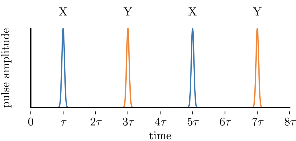
Each cycle of a dynamical decoupling is a sequence of X-Y-X-Y pulses, and each of the four pulses are equally distributed in a cycle. For example, if the idling duration assigned to a cycle is \(8\tau\), each pulse is assigned to the middle of each \(2\tau\) duration. The resulting pulse distribution of a dynamical decoupling cycle is shown in the figure below.

The program below realizes this pattern of the dynamical decoupling sequence. The sequence is shown as a standalone program, but the same sequence can be inserted into any program that has idling qubits.

qubit = 0
idle_duration = 10e-6
n_cycles = 3


@aq.main
def idle_with_dd():
    dd_spacing = idle_duration / (4 * n_cycles)

    drive_frame = device.frames[f"Transmon_{qubit}_charge_tx"]

    pulse.delay(drive_frame, dd_spacing)
    for _ in aq.range(n_cycles):
        x_pulse(qubit)
        pulse.delay(drive_frame, 2 * dd_spacing)
        y_pulse(qubit)
        pulse.delay(drive_frame, 2 * dd_spacing)
        x_pulse(qubit)
        pulse.delay(drive_frame, 2 * dd_spacing)
        y_pulse(qubit)

    pulse.delay(drive_frame, dd_spacing)

The OpenQASM script of the dynamical decoupling program is printed out below.

print(idle_with_dd.build().to_ir())

OPENQASM 3.0;
cal {
    delay[833.333333333333ns] Transmon_0_charge_tx;
}
for int _ in [0:3 - 1] {
    rx(3.141592653589793) $0;
    cal {
        delay[1.666666666667us] Transmon_0_charge_tx;
    }
    rz(-1.5707963267948966) $0;
    rx(3.141592653589793) $0;
    rz(1.5707963267948966) $0;
    cal {
        delay[1.666666666667us] Transmon_0_charge_tx;
    }
    rx(3.141592653589793) $0;
    cal {
        delay[1.666666666667us] Transmon_0_charge_tx;
    }
    rz(-1.5707963267948966) $0;
    rx(3.141592653589793) $0;
    rz(1.5707963267948966) $0;
}
cal {
    delay[833.333333333333ns] Transmon_0_charge_tx;
}

Summary

This example shows you how to use pulse programming to create a program. Just as with a gate-based program, a pulse program in AutoQASM is composed in a function decorated by @aq.main. With AutoQASM, the pulse instructions are automatically added to cal blocks in OpenQASM script, and gate and pulse instructions can be used side-by-side within the same scope of the AutoQASM program.